Plot the Monitor, One Plot per Station

Plot the Monitor, One Plot per Station

plot_monitor(
  x,
  type = c("trend", "intake", "weight", "hours"),
  locations = NULL
)

Arguments

x

Result of run_monitor().

type

"trend" (default), "intake", "weight" or "hours". See Details.

locations

Stations to plot. Default NULL: all.

Value

A data.table with one row per station: location, type, plot (list of ggplot objects), and width and height (cm) that suit the plot when saving it with save_monitor_plots().

Details

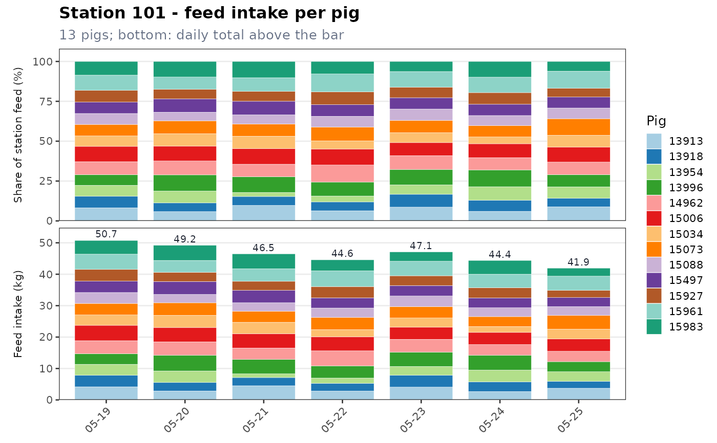
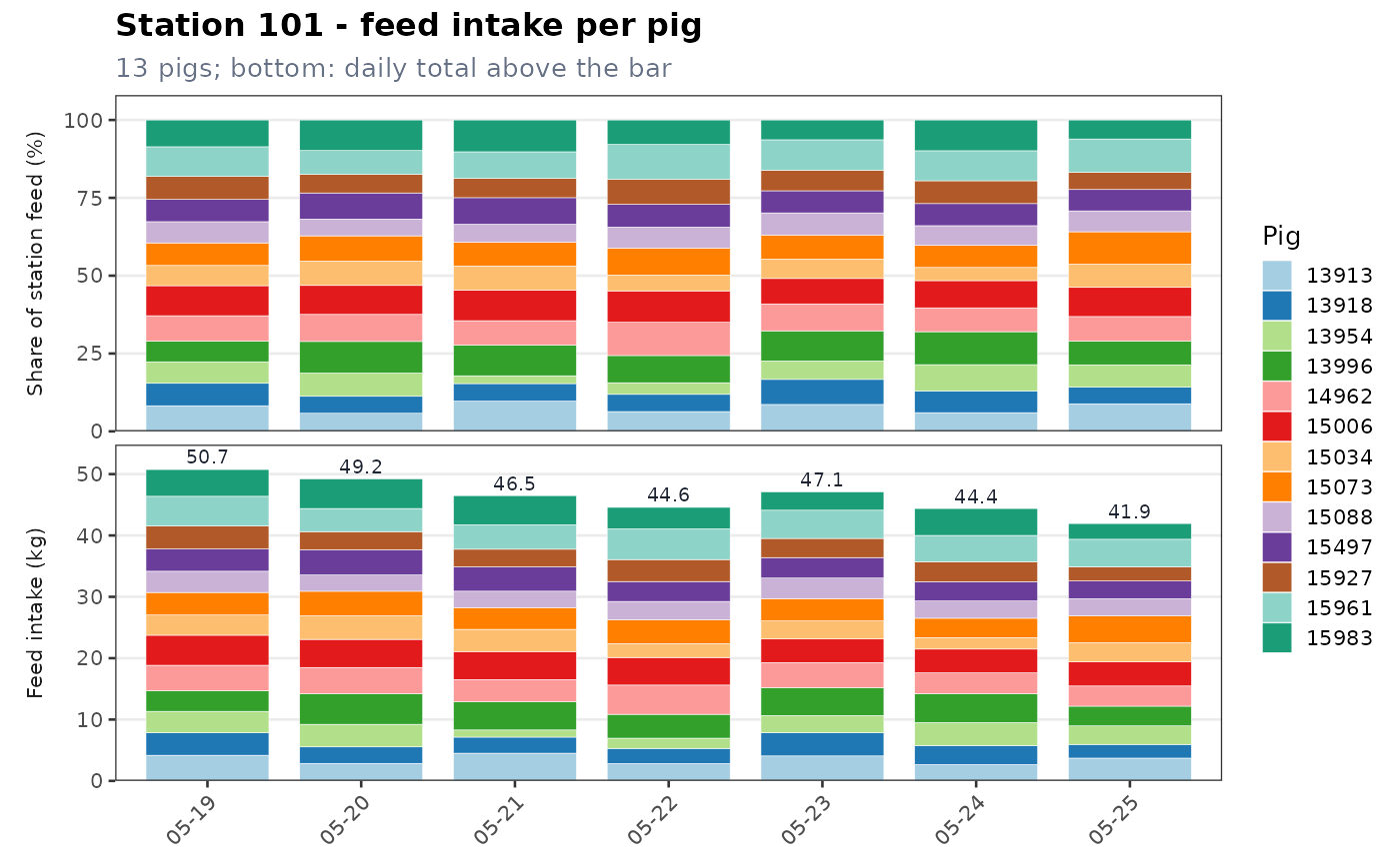
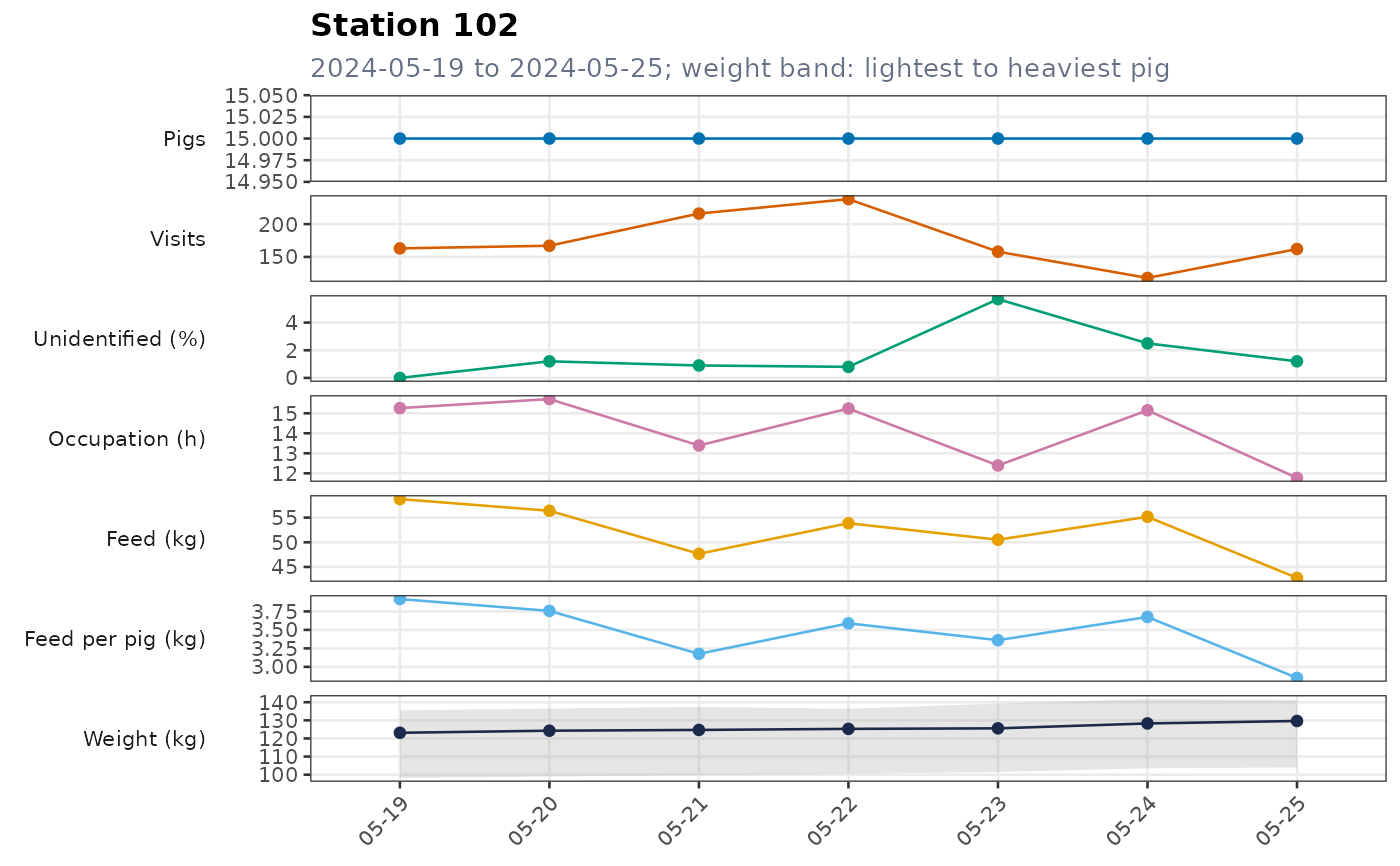
• "trend": pigs, visits, percentage of unidentified visits, occupation time, feed intake, feed intake per pig and body weight on each day of the window. The body weight line is the mean over the pigs of their daily median weight; the band goes from the lightest to the heaviest pig. Days without any visit are shaded red.

• "intake": stacked bars, one colour per pig. Top: the share of each pig in the feed intake of the station that day (%); bottom: its feed intake (kg), with the daily total above the bar (windows of up to 31 days). In the legend, pigs without visit on the last day are marked [no visit] and pigs below low_feed_kg [low feed].

• "weight": box plots of the recorded body weights of each day.

• "hours": visits, occupation time and feed intake per hour of the last day.

See also

save_monitor_plots(), write_monitor_report().

Examples

mon <- run_monitor(tidypptsda::nedap, verbose = 0)
p <- plot_monitor(mon, "intake")
p$plot[[1]]

plot_monitor(mon, "trend", locations = "102")$plot[[1]]

mon <- run_monitor(tidypptsda::nedap, verbose = 0)
plot_monitor(mon, "intake")$plot[[1]]