tidypptsdm
tidypptsdm watches the feeding stations of a pig performance test from day to day. It answers the questions of the daily round: is every station recording, are the transponders read, does every pig still eat, and how did feed intake and body weight develop over the last days?
The data are read and prepared with tidypptsda:
read_station() reads NEDAP or FIRE exports and
prep_visits() turns them into one standard visit table
(feed intake in g, body weight in kg, duration in seconds, unidentified
visits kept with identified = FALSE, pigs moved to another
station resolved). Both functions are re-exported, so
library(tidypptsdm) is enough.
library(tidypptsdm)

mon <- run_monitor(tidypptsda::nedap, days = 7, verbose = 0)
mon
#>
#> ── NEDAP monitor: 2024-05-19 to 2024-05-25 ─────────────────────────────────────
#> ℹ 2 stations, 28 pigs; on 2024-05-25: 366 visits, 84.8 kg feed
#> ✔ No alerts
#> Tables: $stations, $houses, $pigs, $pig_summary, $hours, $alerts. Write them
#> with write_monitor_report() or write_monitor_tables().
Internal helpers
Small internal tools shared by every function of the package:
-
verbosity: exported functions have
verbose = 0/1/2(silent / summary / details), as in tidypptsda; -
input:
as_visits()accepts a folder or files, a raw export, the result ofread_station()or ofprep_visits(), and always returns a copy, so user objects are never modified; -
window:
monitor_window()turnsdaysandend_dateinto the dates of the monitoring window.
One monitoring run
run_monitor() is the function for the daily round. It
prepares the visits once, computes every table over the last
days days and lists the alerts of the last day. Its result
goes to write_monitor_report(),
write_monitor_tables() and plot_monitor().
The window ends on end_date. By default this is the last
day in the data; when that is today, it is the day before, because an
export taken during the day has an incomplete last day.
mon <- run_monitor(tidypptsda::nedap, days = 7)
#>
#> ── Preparing NEDAP visits ──────────────────────────────────────────────────────
#>   Visits read                                31,863
#>   └ unidentified (kept, identified = FALSE)     211    0.7%
#>   └ body weight 0 (set to NA)                   391    1.2%
#> ℹ No pig was seen at more than one station
#> ✔ 30 pigs at 2 stations, 31,863 visits over 97 days 0.1s
#> ℹ No breed column. To use breed in the feed intake model and breed-specific limits, add it with `add_breed()`.
#>
#> ── Monitoring NEDAP stations: 2024-05-19 to 2024-05-25 (7 days) ────────────────
#> ℹ 2 stations, 28 pigs; on 2024-05-25: 366 visits, 84.8 kg feed
#> ✔ No alerts
mon$alerts
#> Empty data.table (0 rows and 6 cols): level,type,location,responder,value,message
head(mon$stations)
#>    location       date n_pigs n_visits n_unidentified pct_unidentified
#>      <char>     <Date>  <int>    <int>          <int>            <num>
#> 1:      101 2024-05-19     13      192              2              1.0
#> 2:      101 2024-05-20     13      201              4              2.0
#> 3:      101 2024-05-21     13      228              2              0.9
#> 4:      101 2024-05-22     13      214              3              1.4
#> 5:      101 2024-05-23     13      234              1              0.4
#> 6:      101 2024-05-24     13      154              1              0.6
#>    occupation_h feed_kg feed_per_pig_kg weight_kg pct_weight_outlier
#>           <num>   <num>           <num>     <num>              <num>
#> 1:        13.88  50.923           3.903    126.83                3.7
#> 2:        13.38  49.585           3.786    128.02                6.6
#> 3:        12.54  46.784           3.576    128.81                7.1
#> 4:        12.63  44.780           3.429    130.49                6.2
#> 5:        13.22  47.120           3.624    131.21                9.0
#> 6:        12.66  44.424           3.415    132.80                7.2
Daily tables
Each table has one row per unit and day of the window, also for days without any visit (counts are then 0). That is what makes a station that stopped recording, or a pig that stopped eating, visible.
Stations
st <- monitor_stations(tidypptsda::nedap, days = 7, verbose = 0)
st
#>     location       date n_pigs n_visits n_unidentified pct_unidentified
#>       <char>     <Date>  <int>    <int>          <int>            <num>
#>  1:      101 2024-05-19     13      192              2              1.0
#>  2:      101 2024-05-20     13      201              4              2.0
#>  3:      101 2024-05-21     13      228              2              0.9
#>  4:      101 2024-05-22     13      214              3              1.4
#>  5:      101 2024-05-23     13      234              1              0.4
#>  6:      101 2024-05-24     13      154              1              0.6
#>  7:      101 2024-05-25     13      204              4              2.0
#>  8:      102 2024-05-19     15      163              0              0.0
#>  9:      102 2024-05-20     15      167              2              1.2
#> 10:      102 2024-05-21     15      216              2              0.9
#> 11:      102 2024-05-22     15      238              2              0.8
#> 12:      102 2024-05-23     15      158              9              5.7
#> 13:      102 2024-05-24     15      118              3              2.5
#> 14:      102 2024-05-25     15      162              2              1.2
#>     occupation_h feed_kg feed_per_pig_kg weight_kg pct_weight_outlier
#>            <num>   <num>           <num>     <num>              <num>
#>  1:        13.88  50.923           3.903    126.83                3.7
#>  2:        13.38  49.585           3.786    128.02                6.6
#>  3:        12.54  46.784           3.576    128.81                7.1
#>  4:        12.63  44.780           3.429    130.49                6.2
#>  5:        13.22  47.120           3.624    131.21                9.0
#>  6:        12.66  44.424           3.415    132.80                7.2
#>  7:        12.30  42.030           3.226    133.57               10.5
#>  8:        15.26  58.752           3.917    123.13                6.1
#>  9:        15.71  56.385           3.757    124.28                8.5
#> 10:        13.39  47.664           3.176    124.70                7.9
#> 11:        15.24  53.857           3.589    125.29                6.8
#> 12:        12.39  50.520           3.361    125.58                6.7
#> 13:        15.15  55.163           3.675    128.28                8.7
#> 14:        11.77  42.784           2.851    129.64               10.0
wide_table(st, "feed_kg")
#> Key: <location>
#>    location  05-19  05-20  05-21  05-22 05-23  05-24  05-25   total
#>      <char>  <num>  <num>  <num>  <num> <num>  <num>  <num>   <num>
#> 1:      101 50.923 49.585 46.784 44.780 47.12 44.424 42.030 325.646
#> 2:      102 58.752 56.385 47.664 53.857 50.52 55.163 42.784 365.125
Houses
A house is a group of stations, named by the first
house_width characters of the station ID.
monitor_houses(tidypptsda::nedap, days = 5, verbose = 0)
#>     house       date n_stations n_pigs n_visits feed_kg feed_per_pig_kg
#>    <char>     <Date>      <int>  <int>    <int>   <num>           <num>
#> 1:      1 2024-05-21          2     28      444  94.448           3.362
#> 2:      1 2024-05-22          2     28      452  98.637           3.515
#> 3:      1 2024-05-23          2     28      392  97.640           3.483
#> 4:      1 2024-05-24          2     28      272  99.587           3.554
#> 5:      1 2024-05-25          2     28      366  84.814           3.025
#>    weight_kg
#>        <num>
#> 1:    126.50
#> 2:    127.62
#> 3:    128.08
#> 4:    130.36
#> 5:    131.39
Pigs
pigs <- monitor_pigs(tidypptsda::fire, days = 7, verbose = 0)
pigs[status != "ok"]
#>    location responder       date n_visits feed_kg occupation_min weight_kg
#>      <char>    <char>     <Date>    <int>   <num>          <num>     <num>
#> 1:      102     35857 2024-02-22        2  -0.012            7.8     118.4
#> 2:      102     35860 2024-02-22        4   0.006            5.6     122.8
#> 3:      102     35861 2024-02-22        4   0.096           12.3     137.2
#> 4:      102     35882 2024-02-22        4   0.300            8.9     131.7
#> 5:      102     35883 2024-02-22        2   0.004            0.5        NA
#>      status
#>      <char>
#> 1: low_feed
#> 2: low_feed
#> 3: low_feed
#> 4: low_feed
#> 5: low_feed
Hours of the day
h <- monitor_hours(tidypptsda::nedap, verbose = 0)
wide_table(h, "n_visits")
#> Key: <location>
#>    location    00    01    02    03    04    05    06    07    08    09    10
#>      <char> <int> <int> <int> <int> <int> <int> <int> <int> <int> <int> <int>
#> 1:      101     3     6     9     4     2     5    10    10    12    17    13
#> 2:      102     9     1     5     5     1     4     6    10     8     9     9
#>       11    12    13    14    15    16    17    18    19    20    21    22
#>    <int> <int> <int> <int> <int> <int> <int> <int> <int> <int> <int> <int>
#> 1:    12     9     4    10    17    15    17    14     9     6     0     0
#> 2:    10     3     1    13    10    10    13    13    13     9     0     0
#>       23 total
#>    <int> <num>
#> 1:     0   204
#> 2: 0 162Wide tables
The daily tables are long: one row per unit and day.
wide_table() turns one column into a table with the units
in rows and the days (or hours) in columns, as in the Excel
workbook.
mon <- run_monitor(tidypptsda::nedap, verbose = 0)
wide_table(mon$stations, "n_visits")
#> Key: <location>
#>    location 05-19 05-20 05-21 05-22 05-23 05-24 05-25 total
#>      <char> <int> <int> <int> <int> <int> <int> <int> <num>
#> 1:      101   192   201   228   214   234   154   204  1427
#> 2:      102   163   167   216   238   158   118   162  1222
wide_table(mon$pigs, "feed_kg")
#> Key: <location, responder>
#>     location responder 05-19 05-20 05-21 05-22 05-23 05-24 05-25  total
#>       <char>    <char> <num> <num> <num> <num> <num> <num> <num>  <num>
#>  1:      101     13913 4.175 2.858 4.514 2.832 4.068 2.665 3.717 24.829
#>  2:      101     13918 3.655 2.685 2.619 2.467 3.792 3.107 2.231 20.556
#>  3:      101     13954 3.505 3.681 1.168 1.664 2.796 3.738 3.015 19.567
#>  4:      101     13996 3.386 4.986 4.590 3.892 4.558 4.698 3.215 29.325
#>  5:      101     14962 4.124 4.278 3.635 4.764 4.075 3.402 3.290 27.568
#>  6:      101     15006 4.894 4.577 4.562 4.497 3.837 3.875 3.923 30.165
#>  7:      101     15034 3.294 3.850 3.612 2.264 2.937 1.878 3.135 20.970
#>  8:      101     15073 3.680 3.995 3.549 3.873 3.648 3.149 4.358 26.252
#>  9:      101     15088 3.458 2.650 2.672 2.994 3.343 2.811 2.815 20.743
#> 10:      101     15497 3.624 4.131 3.971 3.250 3.344 3.148 2.876 24.344
#> 11:      101     15927 3.739 2.937 2.867 3.581 3.118 3.250 2.305 21.797
#> 12:      101     15961 4.846 3.762 3.983 4.999 4.599 4.284 4.502 30.975
#> 13:      101     15983 4.364 4.832 4.750 3.502 2.994 4.385 2.561 27.388
#> 14:      102     13935 3.783 4.279 2.207 3.940 2.575 3.987 3.225 23.996
#> 15:      102     14260 4.488 3.790 2.989 3.132 4.760 4.014 3.035 26.208
#> 16:      102     14730 3.844 3.766 3.379 4.071 3.153 3.602 3.928 25.743
#> 17:      102     14751 2.636 3.173 2.236 2.988 2.839 3.189 1.835 18.896
#> 18:      102     14759 4.083 3.576 3.211 4.122 3.570 3.465 3.282 25.309
#> 19:      102     14903 4.611 3.506 3.795 3.617 4.132 3.535 3.128 26.324
#> 20:      102     14913 4.717 3.582 3.574 4.514 3.040 5.207 3.296 27.930
#> 21:      102     14915 3.571 3.521 2.333 3.225 3.468 2.991 1.609 20.718
#> 22:      102     14937 4.110 5.785 3.734 4.053 4.069 3.896 2.956 28.603
#> 23:      102     14969 5.269 3.881 4.175 3.288 4.418 2.935 3.631 27.597
#> 24:      102     15404 3.659 3.046 3.549 2.379 2.446 4.178 1.751 21.008
#> 25:      102     15496 3.596 4.522 4.474 4.767 3.119 4.265 4.458 29.201
#> 26:      102     15604 3.382 4.139 2.094 3.528 2.636 3.790 2.058 21.627
#> 27:      102     15626 2.869 2.849 2.721 3.019 2.534 2.209 2.590 18.791
#> 28:      102     15649 4.134 2.939 3.170 3.191 3.663 3.869 1.982 22.948
#>     location responder 05-19 05-20 05-21 05-22 05-23 05-24 05-25  total
#>       <char>    <char> <num> <num> <num> <num> <num> <num> <num>  <num>
Plots
plot_monitor() draws one plot per station. There are
five types:
-
"trend": pigs, visits, unidentified visits, occupation time, feed intake and body weight over the window; days without any visit are shaded red; -
"intake": stacked bars of the feed intake of each pig on each day: its share of the station’s feed (top) and kg (bottom), asfid_monitor()of pptsdm drew them; pigs that did not visit or ate too little on the last day are marked in the legend; -
"weight": recorded body weights per day as box plots; -
"hours": visits, occupation time and feed intake per hour of the last day.
mon <- run_monitor(tidypptsda::nedap, verbose = 0)
plot_monitor(mon, "intake")$plot[[1]]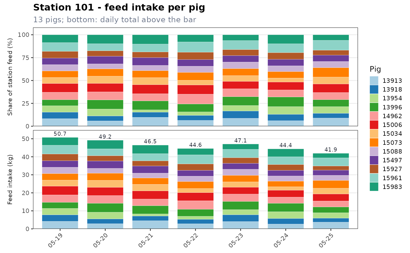
Saving plots
mon <- run_monitor(tidypptsda::nedap, verbose = 0)
dir <- file.path(tempdir(), "monitor_plots")
save_monitor_plots(plot_monitor(mon, "trend"), dir)
#> ✔ Saved 2 of 2 plots to /tmp/RtmptAdiZM/monitor_plots
unlink(dir, recursive = TRUE)
HTML report
write_monitor_report() writes the monitor as a small
offline website, as write_report() does in tidypptsda: an
overview page with the alerts and a table of all stations, then one page
per station with its plots and its pigs. Turn the pages with the arrow
keys and type a pig ID to jump to its station.
mon <- run_monitor(tidypptsda::nedap, verbose = 0)
dir <- file.path(tempdir(), "monitor_report")
write_monitor_report(mon, dir)
#> ✔ Report of 2 stations written to /tmp/RtmptAdiZM/monitor_report/index.html
unlink(dir, recursive = TRUE)
Excel workbook and CSV files
mon <- run_monitor(tidypptsda::nedap, verbose = 0)
dir <- file.path(tempdir(), "monitor_tables")
write_monitor_tables(mon, dir, format = "csv")
#> ✔ Wrote 6 CSV files to /tmp/RtmptAdiZM/monitor_tables
unlink(dir, recursive = TRUE)
Run every day
schedule_monitor() writes an R script that reads the
export folder, runs the monitor and writes the report and the workbook
into a folder named after the last day. On Windows the script is
registered in the Task Scheduler (with the taskscheduleR package). On
Linux and macOS the function prints the line to add with
crontab -e.
folder <- file.path(tempdir(), "exports")
dir.create(folder, showWarnings = FALSE)
data.table::fwrite(tidypptsda::nedap, file.path(folder, "nedap.csv"))
out <- file.path(tempdir(), "monitor_runs")
script <- schedule_monitor(folder, out, days = 7, register = FALSE)
#> ✔ Monitor script written to /tmp/RtmptAdiZM/monitor_runs/tidypptsdm_monitor.R
cat(readLines(script), sep = "\n")
#> # Written by tidypptsdm::schedule_monitor() on 2026-10-31 06:38
#> # Daily monitor of the testing stations: edit the settings below if needed.
#> mon <- tidypptsdm::run_monitor("/tmp/RtmptAdiZM/exports", days = 7)
#> out <- file.path("/tmp/RtmptAdiZM/monitor_runs", format(mon$settings$end_date))
#> tidypptsdm::write_monitor_report(mon, out)
#> tidypptsdm::write_monitor_tables(mon, out, format = "xlsx")
unlink(c(folder, out), recursive = TRUE)